Covid-19 Case Fitting Curves
| Site: | Moodle USP: e-Disciplinas |
| Curso: | Metodos Matematicos da Fisica |
| Livro: | Covid-19 Case Fitting Curves |
| Impresso por: | Utente ospite |
| Data: | quinta-feira, 20 jun. 2024, 08:40 |
Descrição
Last update: 29/08/2020
1. Model Function
Based on data from Covid-19 cases from China, a universal fitting curve is presented. Only four parameters are required to be determined by a given Covid-19 case over a number of days. Under the special condition of reliable mass testing, this curve can indicate the flattening of a given case after its inflection point is reached.
The hyperbolic tangent function,
\begin{equation}
\label{eq:tgh}
Z_{N}(n)=A\tanh(an-b)+C,
\end{equation}
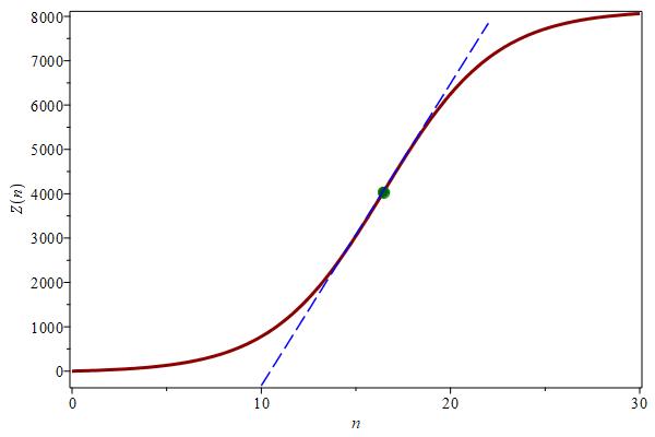
has two desirable features of any Covid-19 case data over the number of days $n$: it is flat at its endpoints and has one inflection point (at $n_{i}=b/a$. Parameter $A$ (or $C=Z(n_{i})$) gives the magnitude of the accumulated cases over $N$ days (amplitude is $2A$). Its steepness is tuned by the slope $a$ of the straight line $an-b$.
Figure 1 shows a typical case for the model function, in which \(A=4086.9\) is the magnitude and $0.170n-2.807$ (dashed line) is its steepness. The green dot is the inflection point ($n_{i}=16.48$).
its steepness (dashed line $0.170n-2.807$).
Parameters $\{A,a,b,C\}$ appearing in the model function were obtained inside Maple and Mathematica by a (local) non-linear fitting minimizing the root mean square (rms) deviation (both worksheet and notebook can be found here and here. All case data points are weighted equally. Case data from every country are available at Worldometer.
Root mean square (rms) deviations shown by inlets in figures belong to the fitted curve $Z_{N}$, where $N$ is the number of days in a given case data. Lower the rms, better the fitting. Residual is the difference between reported and predicted cases, using the last day fitted curve.
Nonetheless, it is important to say that despite the (weak) evidences presented below, any prediction here is not to be taken for granted. Also, this is a simple exercise of reconversion, since I am not an expert in the Statistics Science. See Refs.[1]-[4] for more accurate fitting schemes.
2. Closed Cases
Closed Cases show some countries having a flattening in their Covid-19 curves. This is the case of China. South Korea had two waves of Covid-19 cases, with the last wave closing.
2.1. China
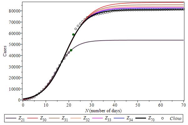
Figure 2 shows the case curves for the complete Covid-19 case data from China. The whole data seems to have a subseries described by the curve \(Z_{21}\) (the violet curve), obtained using the first 21 days, which indicates a (local) flattening of the cases over two weeks (around 53,700 cases). In spite of this curve $Z_{21}$ being a false lead in searching for the case flattening, since we know the whole history, it has all features of a typical (complete) case curve. In fact, a close analysis in this subseries shows an inflection point around $N=14$. Also, while the nearest case curves $Z_{N\leq 21}$ approach $Z_{21}$ in an oscillatory way, all case curves $Z_{N\geq 23}$ approach monotonically the global case curve $Z_{70}$ (the black curve in Figure 2), obtained using the first 70 days in the case data from China, which indicates a flattening around 81,000 cases. Therefore, the (black) curve $Z_{70}$ shown in Figure is the lower limit for all curves $Z_{N\geq 22}$ and has its inflection point around $N=21$. All curves $Z_{N\geq 29}$ converge monotonically and rapidly to $Z_{70}$, giving a 10 days prediction for the (global) flattening. Best parameters for these two curves are shown in Table Par-China.
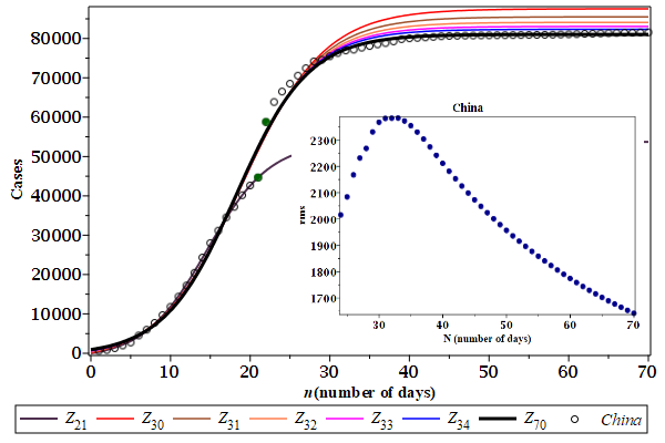
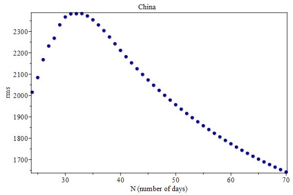
We have learned that the case curves $Z_{N}$ obtained after the inflection point converge monotonically, in an increasing speed, to the global case curve. Of course, mass testing is presumed. Figure rms-China shows the root mean square (rms) deviations of each case curve $Z_{N\geq 22}$, confirming the monotonic convergence.
Some questions. What did happen at day 22? Was it an increase in the total tests? Or is this jump in the number of cases from day 21 to the day 22 (see the solid green circles in Figure Cases-China) a typical feature of the global case curve around its inflection point (where the rate of change is maximum)?
2.2. South Korea
South Korea has a case data with two series: (a) day 1 to 30 , \(1\leq N\leq 30\), fitted curve $Z_{a}$ (green line in Figure 3), and (b) day 31 and after ($N\geq 31$), fitted curve $Z_{b}$ (blue line in Figure 3). These two series are quite different from the Chinese two subseries, where there is a global fitting curve (see Figure 2). As we can see in Figure 3, the thin curve ($Z_{79}$) does not fit properly the whole data. A second wave of Covid-19 cases is in progress in South Korea (curve $Z_{b}$ in Figure 3). Fortunately, this second wave is flattening. The inlet in Figure 3) shows the root mean square (rms) deviations for the last $N$ days from the curve with the full data (upper grey dots) and the curve $Z_{b}$ from the second wave (lower blue dots).

An very important lesson can be learned here: a second wave of infections can come quickly.
2.3. New Zealand
New Zealand seems to have reached a global flattening, as we can see in Figure 4. Its case data has one jump at day 31 to 32 and its root mean square deviations are getting smaller (see inlet in Figure 4). There are repeated data resembling jumps at days 19-22 and 25-28, but probably they are not.
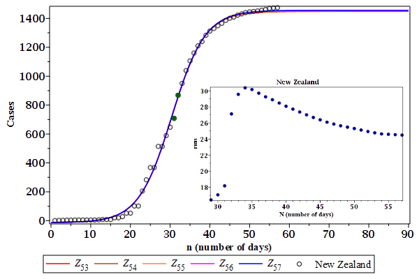
There is a growing oscillation in the case data around the last day fitted curve which can leads to a false flattening, like the case data from South Korea. This growing oscillation can be also the indicative of a second wave in course.
3. Almost Closed Cases
Almost Closed Cases show some countries Covid-19 case data close to their global flattening. New waves of new infections are not ruled out. In fact many case data shown here require a multi-wave analysis.3.1. Spain
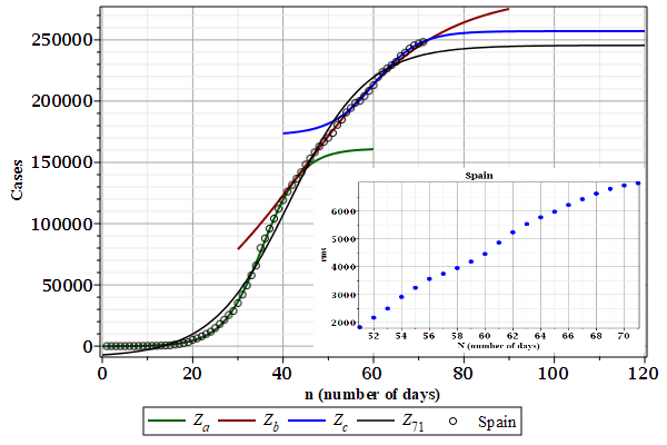
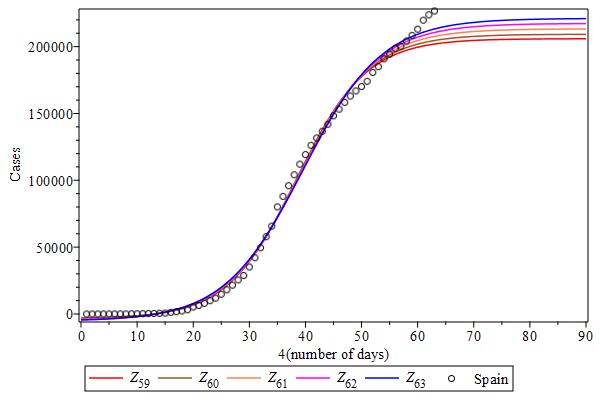
The case data from Spain seems to have three harmonics (or waves). The last wave $Z_{c}$ (blue line) seems to be reaching its flattening. The root mean square (rms) deviations in the inlet were calculated by the fitted curve \(Z_{71}\) using the whole case data.
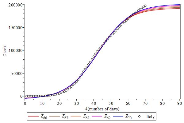
3.2. Italy
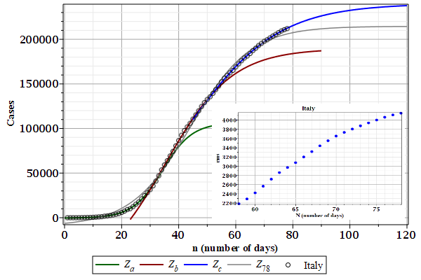
The case data from Italy seems to have three harmonics (or waves). The last wave $Z_{c}$ (blue line) is still growing. The root mean square (rms) deviations in the inlet were calculated by the fitted curve \(Z_{78}\) using the whole case data.
3.3. France
3.4. Iran
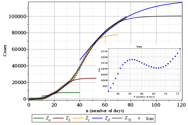
The case data from Iran seems to have four harmonics (or waves). The last wave $Z_{d}$ (blue line) is still growing. The root mean square (rms) deviations in the inlet were calculated by the fitted curve \(Z_{76}\) using the whole case data.
3.5. Australia
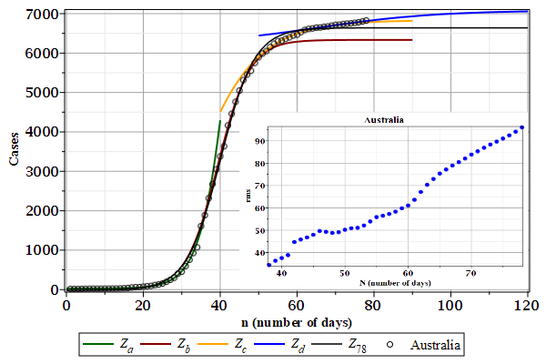
The case data from Australia seems to have four harmonics (or waves). The last wave can keep growing. The root mean square (rms) deviations in the inlet were calculated by the fitted curve \(Z_{78}\) using the whole case data.
4. More Cases
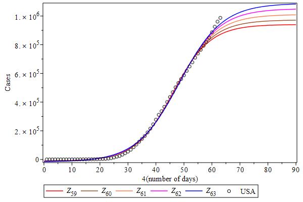
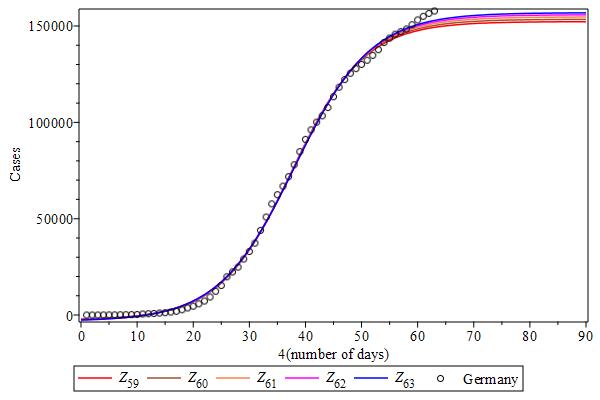
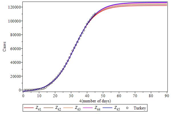
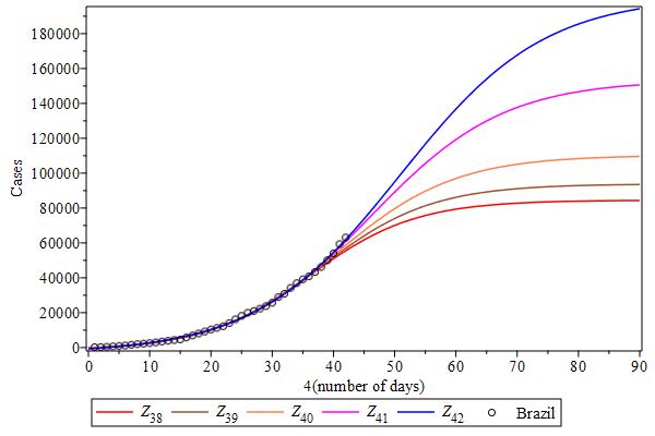
Let us try to analyze case data from other countries based on what we have learned from the Chinese case data, under the model function. Figure Cases-USA shows the case curves over the last five days for the USA case data. Since these curves are ordered, with the last day (blue) curve at the top, and quite distant from each other at the flattening region, it shows (probably) that the inflection point was not reached yet, but it could be close. The case curves from Spain, Italy, Germany, UK and Turkey have these same features (see Figures Cases-Spain to Turkey). Russia and Brazil seem to be far away from their inflection points (see Figures Cases-Russia to Brazil).
What about the planet Earth? Figure Cases-World shows the world case data. It seems to be far away from the inflection point. Better stay at home.
4.1. Jumps
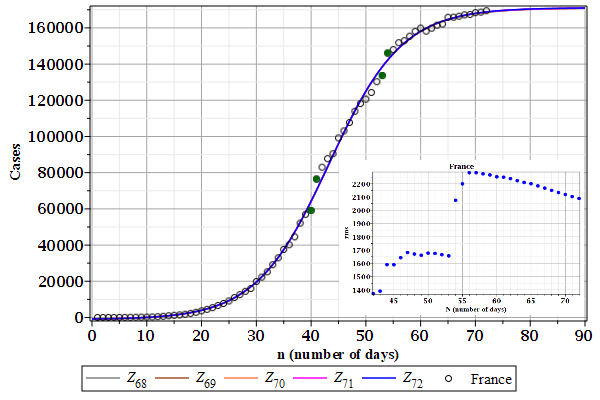
Jumps. The case data from France shown in Figure Cases-France has two jumps: at day 40 to 41 and at day 53 to 54 (see the solid green circles). Two subseries is something new. The case data from UK seems to have one jump at day 45 to 46 (see the solid green circles Figure Cases-UK), but it can be diminished by the growth in case data.
4.2. Flattenings
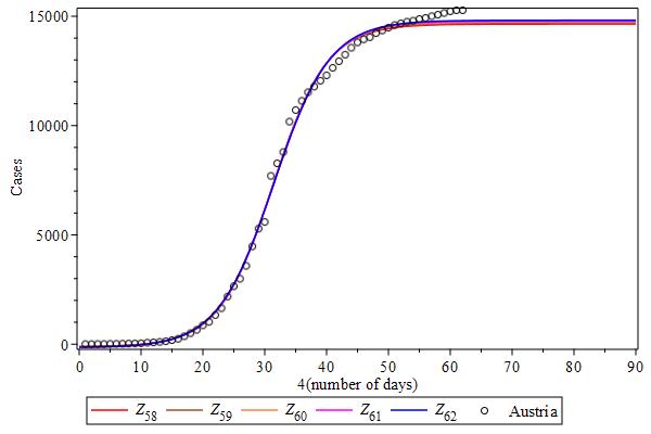
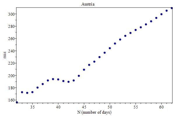
France and Iran have case curves indicating a possible flattening (the last curve is a lower limit), as shown in Figures Cases-France and Iran. Reinforcing that, for Iran only, Figure rms-Iran shows that the root mean square (rms) deviation seems to have reached its maximum. However, these flattenings could be false leads due to oscillations in the case data. Australia and Austria also seems to have false flattenings, since their rms have not reached any maximum (see Figures Cases-Auatralia -- rms-Austria).
New Zealand seems to have reached a global flattening, as we can see in Figures Cases-New Zealand and rms-New Zealand. Its case data has one jump at day 31 to 32 and its root mean square deviations are getting smaller.
4.3. Residuals
Residuals. Residuals are the difference between reported and predicted cases, using the last day fitted curve. There are growing oscillations in the residuals from US, Spain, Italy and Germany case data. Iran has the most regular oscillations in their residuals, as shown in Figure res-Iran. These oscillations superpose a modulation in the case data, which can not be accounted by the hyperbolic tangent in the model function. Perhaps a q-deformed hyperbolic tangent could delivery a better response, using the deformation parameter to control its steepness.
4.4. Two Series
South Korea has a case data with two series: (a) day 1 to 30 (\(1\leq N\leq 30\)), fitted curve $Z_{a}$ (green line in Figure Cases-South Korea), and (b) day 31 and after ($N\geq 31$), fitted curve $Z_{b}$ (blue line in Figure Cases-South Korea). These two series are quite different from the Chinese two subseries, where there is a global fitting curve (see Figure Cases-China). As we can see in Figure Cases-South Korea, the thin red curve ($Z_{73}$) does not fit properly the whole data. A second wave of Covid-19 cases is in progress in South Korea (blue line $Z_{b}$ in Figure Cases-South Korea). Fortunately, this second wave is flattening. An important lesson can be learned here: a second wave of case infections can come very fast.
5. Non-linear fitting
Parameters \(\{A,a,b,C\}\) appearing in the model function were obtained inside Maple and Mathematica by a (local) non-linear fitting minimizing the least-squares error (both worksheet and notebook can be found here and here). An update pdf version can be found here. All case data points are weighted equally. Case data from every country are available at Worldometer (www.worldometers.info), Coronavirus (www.worldometers.info/coronavirus).
6. References
[1] S. Maltezos, Parametrization Model Motivated from Physical Processes for Studying the Spread of COVID-19 Epidemic. arXiv:2004.05992v2 [physics.soc-ph] (2020).
[2] P. Girardi et al., Robust inference for nonlinear regression models from the Tsallis score: application to Covid-19 contagion in Italy. arXiv:2004.03187v2 [stat.AP] (2020).
[3] M. A. V. Arias, Using generalized logistics regression to forecast population infected by Covid-19. arXiv:2004.02406v1 [q-bio.PE] (2020).
[4] J. Kumar and K. P. S. S. Hembram, Epidemiological study of novel coronavirus (COVID-19). arXiv:2003.11376v1 [q-bio.PE] (2020).
\(
\begin{thebibliography}{10}
\bibitem{Maltezos}
S. Maltezos,
\newblock{Parametrization Model Motivated from Physical Processes
for Studying the Spread of COVID-19 Epidemic}.
\newblock \href{https://arxiv.org/abs/2004.05992}{arXiv:2004.05992v2
[physics.soc-ph]} (2020).
\bibitem{Girardi}
P. Girardi \textit{et al.},
\newblock{Robust inference for nonlinear regression models from the
Tsallis score: application to Covid-19 contagion in Italy}.
\newblock \href{https://arxiv.org/abs/2004.03187}{arXiv:2004.03187v2
[stat.AP]} (2020).
\bibitem{Arias}
M. A. V. Arias,
\newblock{Using generalized logistics regression to forecast
population infected by Covid-19}.
\newblock \href{https://arxiv.org/abs/2004.02406}{arXiv:2004.02406v1
[q-bio.PE]} (2020).
\bibitem{Kumar}
J. Kumar and K. P. S. S. Hembram,
\newblock{Epidemiological study of novel coronavirus (COVID-19)}.
\newblock \href{https://arxiv.org/abs/2003.11376}{arXiv:2003.11376v1
[q-bio.PE]} (2020).
\end{thebibliography}
\)
7. Figures
Use left panel to navigate.
7.1. China
| Cases-China |
rms-China |
|---|---|
 |
 |
7.2. USA-Spain
| Cases-USA | Cases-Spain |
|---|---|
 |
 |
7.3. Italy-Germany
| Cases-Italy |
Cases-Germany |
|---|---|
 |
 |
7.4. UK-Turkey
| Cases-UK | Cases-Turkey |
|---|---|
 |
 |
7.5. Russia-Brazil
| Cases-Russia | Cases-Brazil |
|---|---|
 |
 |
7.6. Austria
| Cases-Austria | rms-Austria |
|---|---|
 |
 |